Graduate school
Coursework
USC
M.S. Aerospace Engineering
5
Graduate courses, 2025–2027
Combustion
AME 513a / 513b · Fall 2025 – Spring 2026 · University of Southern California
Python
Analysis
Wrote the Cantera scripts that ran the flame, stretch, and detonation cases.Cantera
Analysis
Used Cantera throughout to simulate premixed and non-premixed flames, then paired those runs with classical analysis.Flame structure
Analysis
Extracted species profiles, heat-release rate, flame thickness, and laminar flame speed from freely propagating flames.Chemical kinetics
Analysis
Sensitivity analysis on rate-controlling steps, plus thermal versus prompt NOx and soot conditions.Turbulent flow
Analysis
Estimated Kolmogorov and Taylor scales for jet flames and placed the cases on the Borghi–Peters regime diagram.
Course description
In Combustion I spent the semester learning how flames work from the inside out, then applying that in practice with Cantera. I started with the thin structure of a freely propagating premixed flame, then added stretch and turbulence. I paired those simulations with classical analysis so I could go from a plot to a clear explanation of why a flame thickens or extinguishes.
Core competencies
- Computed freely propagating /air, /air, and /air flames across equivalence ratio and pressure, then extracted species and radical profiles, heat-release rate, key reaction rates, flame thickness versus reaction-zone thickness, , and
- Ran sensitivity analysis to find the rate-controlling kinetic steps and mapped the conditions that increase and soot
- Stretched twin premixed /air and /air flames and non-premixed –air flames in counterflow, tracked , found , and explained the trends with Lewis number and differential diffusion
- Separated thermal versus prompt in the stretched non-premixed cases
- Estimated turbulence Reynolds number, dissipation, Kolmogorov and Taylor scales, and Kolmogorov time for methane–air jet flames, then placed lab and practical setups on the Borghi–Peters regime diagram
Deep diveFlame structure, stretch, turbulenceOpenClose
Freely propagating · Cantera
Flame structure
I simulated freely propagating premixed flames using Cantera for ethane, ethylene, and acetylene in air, sweeping equivalence ratio and pressure. As shown below, the fuel and oxygen sit flat in the unburned gas, then drop through a thin consumption zone. Radicals and heat release peak within the consumption zone, and in my simulations I found that added pressure continuously compresses the consumption zone.
- Acetylene is the fastest of the three. Ethane is the slowest. That ranking holds in and in .
- Ethane and ethylene peak near stoichiometric and fall off rich. Acetylene keeps climbing on the rich side.
- Mass burning rate still rises with pressure even as flame speed falls, because unburned density wins.
- Sensitivity is dominated by and . High pressure shifts weight toward termination.
- Thermal tracks temperature and is strongest near stoichiometric. Soot wants rich, hot acetylene.
Twin counterflow
Stretch and Lewis number
I extended twin premixed flames in counterflow, followed by a methane–nitrogen versus air diffusion flame. Stretch represents the strain that opposing jets apply to the reaction zone. Its effect on peak temperature depends on which species is deficient and the rate of its diffusion. The form of versus stretch already indicates whether the Lewis number is aiding or hindering the process.
- Lean hydrogen: fuel is deficient and it is the fast diffuser (). Preferential diffusion feeds into the reaction zone, so rises at first. Then stretch wins and the flame dies.
- Rich hydrogen: oxygen is deficient and it is the slow diffuser. falls from the first step, but the flame holds on longer.
- Propane flips the story. Lean propane is a heavy, slow fuel (), so stretch only hurts. Rich propane lets the faster oxygen help, and the flame is much more stretch-resistant.
- Non-premixed methane lives where the fluxes meet stoichiometry, on the air side of stagnation. Diluting the fuel drops and kills stretch resistance. Full chemistry puts a peak at the flame. Thermal-only is lower and falls off faster as residence time shrinks.
Estimated, then placed on Borghi–Peters
Turbulent scales
I estimated the turbulence Reynolds number, dissipation, Kolmogorov and Taylor scales, and Kolmogorov time for methane–air jet flames at the nozzle and within the hot gas. Viscosity increases by more than an order of magnitude once the gas reaches flame temperature, so a jet appearing turbulent at the exit may lie near the laminar edge where heat release occurs. I then positioned several laboratory and practical premixed configurations on the Borghi–Peters diagram.
- A small, fast jet loses most of its turbulent Reynolds number in the hot gas because drops and rises.
- A larger, slower jet still looks turbulent at the flame. Its Kolmogorov length is centimeters, not microns.
- A grid-stabilized flame sits in wrinkled flamelets. A bluff-body duct sits in corrugated flamelets. A small high-speed jet chamber can cross into thin reaction zones.
Compressible Gas Dynamics
AME 511 · Spring 2026 · University of Southern California
Shock relations
Analysis
Rankine–Hugoniot, oblique shocks, reflections, and full shock-tube state calculations.Nozzle theory
Fluids
Rocket-nozzle exit conditions and supersonic wind-tunnel design from the area–Mach relation.CFD
Analysis
3-D rotating-frame propeller study in Earth, Mars, and Titan atmospheres — same blade, different Mach.
Course description
In Compressible Gas Dynamics, I applied conservation laws and shock/expansion relations to study wave propagation and discontinuities. Starting with continuum acoustics, I progressed through finite-amplitude waves and the method of characteristics to shocks, expansions, and nozzles in propulsion and high-speed flight. Combining calculations with classical analysis, I used jump conditions and – diagrams to explain shock steepening, smooth expansion fans, and Mach-number control in nozzles.
Core competencies
- Derived the thermodynamic closures and conservation statements for a calorically perfect gas, then used them on a piston-driven isentropic compression and on isothermal versus isentropic discharge from a rigid tank
- Computed Pitot-tube readings for subsonic and supersonic flight, derived the Hugoniot equation from the Rankine–Hugoniot relations, and found the maximum isentropic velocity from a reservoir
- Solved the –– relation for oblique shocks, wall reflections, opposite-family shock intersections, and a symmetric expansion–compression dip
- Calculated rocket-nozzle exit Mach number, temperature, density, and velocity, and the design numbers for a supersonic wind tunnel
- Tracked a moving normal shock in laboratory and shock-fixed frames, then reconstructed the full shock-tube wave system (incident shock, contact surface, expansion fan, reflected shock) including the density ratios and
- Applied linearized theory to a flat plate at angle of attack, compared lift, drag, and moment coefficients with exact shock-expansion theory, and mapped the relative error with angle of attack and Mach number
- Ran a 3-D rotating-frame CFD study of a high-speed propeller in Earth, Mars, and Titan atmospheres, extracting relative Mach and pressure at , , and span and showing how and density send the same blade supersonic on Mars and subsonic on Titan
Deep diveHigh-speed propeller in Earth, Mars, and Titan atmospheresOpenClose
AME 511 · Group 1 · Spring 2026
High-speed propeller
I worked with a four-person team on a 3-D rotating-frame CFD study of a high-speed propeller. Local speed is , so the hub can sit in weakly compressible flow while the tip goes through Mach 1. We ran the same geometry at RPM in Earth, Mars, and Titan atmospheres. The only things that changed were , , , , and .
- 35,000 RPM
- Operating speed
- 50 / 75 / 100%
- Spanwise slices
- 3 atmospheres
- Earth, Mars, Titan
- Orthogonal slices at , , and span are how I tracked Mach number and static pressure from hub to tip
- NASA used the same rotating-frame approach for Ingenuity’s rotors in thin Martian air
Atmosphere properties
Earth, Mars, and Titan
Identical means identical tip speed. Mach number is that tip speed over the local speed of sound, . I used each atmosphere’s , , , , and gas constant so the Mach field and the pressure loading could move independently.
- Mars is cold , so is low and the blade goes more supersonic, but and are so low that the loading stays tiny
- Titan is a dense, cold column. Mach stays subsonic and the pressure force is the largest of the three
- Earth is the baseline: weakly supersonic at the tip, moderate loading

Earth
Air · sea level
- 288 K
- 101.3 kPa
- 1.23 kg/m³
- 1.4
- MW
- 28.97
M_tip ≈ 1.03
Weakly supersonic tip. Baseline loading.
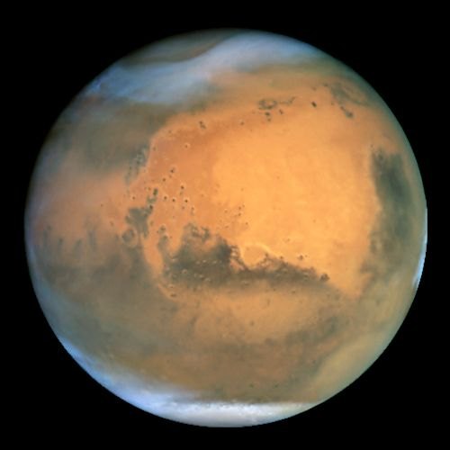
Mars
CO₂ · near-surface
- 210 K
- 0.60 kPa
- 0.015 kg/m³
- 1.3
- MW
- 41.01
M ≈ 1.05–1.12
Highest Mach, weakest pressure loading.

Titan
Dense N₂ · near-surface
- 94 K
- 146 kPa
- 5.3 kg/m³
- 1.4
- MW
- 28.01
M ≈ 0.82–0.91
Entire blade subsonic. Strongest loading.
Mesh and solver
Moving reference frame
The production setup is a two-cylinder moving-reference-frame mesh: an inner rotating zone around the blade and a stationary outer cylinder. About 491k elements, max skewness . We ramped RPM at a time from rest to , first-order, then finished second-order.
- 491k
- Production mesh
- 1.9%
- Mass-flux error, 2-cyl
- 2.85M
- Refinement check
- A single cylindrical domain with a rotating wall would not converge. Residuals jumped at every RPM step, mass flux diverged, and a negative-pressure pocket formed at the outlet
- Interface mass-flux error on the two-cylinder mesh was about
- A M refined mesh showed the same Mach pattern. The student-license cap kept us on the coarse mesh for the atmosphere sweep
- The gas is calorically perfect. The flow is inviscid, steady in the rotating frame, and isentropic except across shocks
Mach and pressure
Earth, hub to tip
On Earth I extracted relative Mach and static pressure at three spanwise stations.
- Mid-span is high-subsonic. Peak relative Mach about , with mild pressure change across the blade
- At span the flow is transonic, , and the pressure gradients get sharper
- At the tip the relative flow is weakly supersonic, , and the pressure jump is the strongest of the three stations
- Compressibility grows from hub to tip. Shocks show up first at the outermost station
3-D field
Pathlines and tip vortices
The spanwise slices are 2-D cuts of a 3-D flow. Relative-velocity pathlines show the tip vortex and the radial pumping you expect from a rotating blade.
- Treating the propeller as an inviscid wall forces the flow to run parallel to the surface, so the solver over-speeds around curvature and the suction peak on the convex face drops out
- That was an acceptable cost to isolate shock and Mach-number trends
- Centrifugal three-dimensionality and the trailing vortex mean a given slice is never a pure problem
Earth, Mars, Titan
Results across atmospheres
I ran the same blade and the same rotation rate in all three atmospheres so the only change was the speed of sound and the density.
- Earth: walks from at mid-span to at the tip
- Mars: colder, heavier puts every slice higher, about to . Highest Mach, weakest pressure loading
- Titan: entirely subsonic, –, and still produces the largest pressure force because the atmosphere is dense
- Atmosphere changes the Mach field through and the loading through and
- A calorically perfect, inviscid gas is enough to see that split. Real and thermodynamics, and viscosity, would likely stretch the differences further
- Pick tip speed for the local speed of sound, then check that the loading you need still exists in that atmosphere
Entry and Landing Systems for Planetary Exploration
ASTE 577 · Fall 2026 · University of Southern California
MATLAB
Analysis
Used MATLAB and Excel to size the EDL stack, from heat load and timeline through the landing sequence.Decelerators
Fluids
Worked aerodynamic decelerators as part of the EDL stack, alongside aerothermodynamics and landing attenuation.Flight computer
CAD / hardware
Built an EDL sequence with timings, comms, and fault response on a Raspberry Pi — temperature, accel, landing trigger, and transmit.Systems engineering
People
Coordinated with Team Discovery to vet a landing system, from research briefs through the term project.
Course description
In the Entry and Landing Systems class, I learned about the process a vehicle undergoes from approach to landing on a safe surface. I applied this knowledge by using MATLAB and Excel for sizing and a Raspberry Pi as the flight computer. The course began with an exploration of historical EDL missions and the causes of TPS failures. I then delved into atmospheric flight mechanics, aerodynamic decelerators, and landing attenuation, analyzing case studies from Mars, Venus, and Titan. Additionally, I led a group of six people in designing a mission, where we transitioned from creating heat-load or timeline plots to providing clear explanations of why specific landing methods, such as heat shields, parachutes, or propulsive landings, were appropriate for each celestial body.
Core competencies
- Walked heritage EDL architectures and mapped physical versus organizational failure onto entry-system requirements
- Sized the stack across aerothermodynamics, decelerators, landing attenuation, and telecom / C&DH, not just the heat shield
- Built an EDL sequence with timings, comms, and fault response on a Raspberry Pi (temperature, accel, landing trigger, transmit)
- Wrote Level 1 requirements and a science traceability matrix for a unique surface measurement, then closed the architecture at the end of the semester
- Coordinated with Team Discovery to vet a landing system, from research briefs through the term project
Deep diveIn developmentOpenClose
Human Spaceflight
ASTE 524 · Fall 2026 · University of Southern California
ConOps
Test ops
Concept of operations: how a system is meant to be run, including roles, sequence, modes, and decision points.Design Reference Mission
Analysis
Turned the Ares Program DRM into capacity, cadence, transit-time, landing, and Earth-return criteria the transportation system had to meet.Human rating
People
Mapped NPR 8705.2C tenets (accommodate, utilize, protect) into abort windows, failure tolerance, onboard autonomy, safe haven, and SPE shelter.Life support / safe haven
Fluids
Four-crew safe haven and a solar particle event shelter reachable in 30 minutes, plus 30 days of zero Earth contact.Crew vehicles
CAD / hardware
Two flight vehicles and three launches per opportunity: cargo Starship plus tanker, and Pathfinder on an augmented STS stack.
Course description
In Human Spaceflight, I gained a comprehensive understanding of the engineering, technologies, and systems essential for human spaceflight. I applied this knowledge to lead a group project focused on designing a habitat and crew transfer to Mars. I started by exploring space environments and crew accommodations. Then, I expanded to include life support systems, launch and entry procedures, rendezvous and docking operations, and extra-vehicular activities. By integrating these systems with mission operations and safety protocols, I successfully transitioned from establishing a Need/Goals/Objectives statement and a Design Reference Mission to developing a Concept of Operations that could be implemented by a viable transportation architecture.
Core competencies
- Wrote Need, Goals, and Objectives for a human Mars program that stay short at the top and measurable in the objectives, without locking a vehicle solution early
- Turned the Ares Program Design Reference Mission into capacity, cadence, transit-time, landing, and Earth-return criteria a Crew and Cargo Transportation System had to meet
- Mapped NASA Procedural Requirements 8705.2C human-rating tenets (accommodate, utilize, protect) into abort windows, failure tolerance, onboard autonomy under light-time delay, safe haven, and solar particle event shelter requirements
- Built a phase-by-phase Concept of Operations (cargo ahead of crew, Earth parking-orbit checkout, Trans-Mars Injection, cruise, Mars capture, landing within 3 km of the base, surface transfer, ascent, and CONUS return) with labeled contingencies from pad escape through abort land landing
- Kept the design as one crewed transportation system: habitat stayed out of scope, architecture choices deferred to ConOps rather than the Need
Deep diveIn developmentOpenClose
Spacecraft System Design
ASTE 520 · Fall 2026 · University of Southern California
Requirements
Test ops
Turned the instructor RFP into testable mission requirements before we sized a subsystem.ConOps
Test ops
Concept of operations: how a system is meant to be run, including roles, sequence, modes, and decision points.Mass & power
Analysis
Kept living first-order mass, power, Δv, data, and pointing budgets with named margins.
Course description
In Spacecraft System Design, I developed and applied the skills needed to create a complete lunar communications architecture from mission concept through first-order subsystem design to a closed vehicle. I translated mission needs into clear requirements and a concept of operations, then progressed through payload definition, orbit selection, propulsion, thermal and power management, structural design, avionics, and attitude control. I evaluated cost, risk, and design feasibility against the mission objectives, ensuring the proposed architecture met the original RFP. I also performed system-level trades to understand how design decisions—such as mass budgets and Δv requirements—drove changes across subsystems and validated the overall vehicle solution.
Core competencies
- Translated an RFP into testable mission requirements and a ConOps with phases, modes, and a first-cut verification path
- Built and kept living first-order mass, power, Δv, data, and pointing budgets with named margins
- Sized the major bus subsystems (payload, propulsion, thermal, EPS, structures and mechanisms, C&DH / telecom / ground, ADCS) and tracked the interfaces between them
- Ran architecture trades on orbit, propulsion type, configuration, and pointing, and revised earlier choices when later analysis said so
- Closed a conceptual design against cost, risk, I&T / V&V, and RFP compliance, and said whether it was credible enough to proceed